Large scale L1 feature selection with Vowpal Wabbit

The job salary prediction contest at Kaggle offers a highly-dimensional dataset: when you convert categorical values to binary features and text columns to a bag of words, you get roughly 240k features, a number very similiar to the number of examples.

We present a way to select a few thousand relevant features using L1 (Lasso) regularization. A linear model seems to work just as well with those selected features as with the full set. This means we get roughly 40 times less features for a much more manageable, smaller data set.

What you wanted to know about Lasso and Ridge

L1 and L2 are both ways of regularization sometimes called weight decay. Basically, we include parameter weights in a cost function. In effect, the model will try to minimize those weights by going “down the slope”. Example weights: in a linear model or in a neural network.

L1 is known as Lasso and L2 is known as Ridge. These names may be confusing, because a chart of Lasso looks like a ridge and a chart of Ridge looks like a lasso.

L1 / Lasso vs. L2 / Ridge

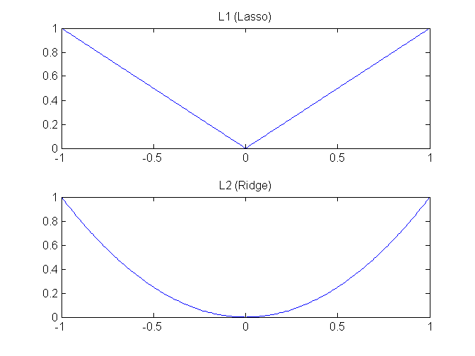
For L1 we use absolute values of weights and for L2 squared values. Therefore, L1 tends to produce relatively few features with the rest set to zero. L2 will select more features and many of them will be close to zero. Lasso is useful for feature selection, while Ridge usually just acts as regularization.

Why Lasso

Do you want a testimonial for using Lasso? Take a look at Practical machine learning tricks from the KDD 2011 best industry paper:

Throw a ton of features at the model and let L1 sparsity figure it out

Feature representation is a crucial machine learning design decision. They cast a very wide net in terms of representing an ad including words and topics used in the ad, links to and from the ad landing page, information about the advertiser, and more. Ultimately they rely on strong L1 regularization to enforce sparsity and uncover a limited number of truly relevant features.

Now for downsides. Francis Bach says that the Lasso is usually not model-consistent and selects more variables than necessary [PDF]. The latter generally is not a problem for us, as we’d rather capture all important ones than leave a few out.

The data

Below are dimensionalities for each column in the data set. As you can see, most features come from job title and description (both bag of words) and from company names (categorical). We will filter the features for these columns and leave the others intact.

Title:             18611
FullDescription:  199613
Loc1:                  1
Loc2:                 20
Loc3:                181
Loc4:               1329
Loc5:               1325
ContractType:          3
ContractTime:          3
Company:           20813
Category:             29
SourceName:          168

We use parsed, hierarchical locations (Loc1…Loc5). You can get them using update_locations_fixed.py script. Loc1 is always “UK”, so you can get rid of this column.

The plan

train to satisfaction
turn L1 regularization on and tune to get the score close to the previous one
run vw-varinfo with the found settings
convert the data to libsvm format - use only selected features

The first point is straightforward - we already have a model from Predicting advertised salaries. Now we’d like to achieve the same, or at least similiar result, only with L1 regularization on. That means using only a subset of features, hopefull a small subset. We tune and when we get the settings needed for achieving this result, we run Vowpal Wabbit using a wrapper called vw-varinfo.

vw-varinfo produces output like this:

FeatureName                HashVal   MinVal   MaxVal    Weight   RelScore
^bread                      220390     0.00     2.00   +0.0984     55.36%
^icecream-sandwich           39873     0.00     1.00   +0.0951     53.44%
^snapple                    129594     0.00     2.00   +0.0867     48.61%

RelScore is what interests us. After Lasso, most of these values should be 0.00%. We delete them by hand in a text editor to retain only the features with non-zero RelScore and then we use this file as an input for the script converting the data.

Using vw-varinfo is also nicely described in a StatsExchange post about finding the best features. The twist there is detecting an interaction of features with -q.

In practice

Note that if you want to produce a submission file, as opposed to perfroming validation, you need to join train and test files before converting them to VW format. It is described in the previous post about this competition. We’re just doing validation and get MAE = 6638 with --l1 0.0000001.

After conversion, the first line of training data looks like this:

Apparently the amount of L1 regularization needed is rather small:

vw -c -k --passes 13 --l1 0.0000001 data/Train.vw

The -k options means “kill the cache” and is useful if you put your new data in the same directory as before. By default VW will use an existing cache. Here’s a sample of output for validation and then for the full set:

average    since         example     example  current  current  current
loss       last          counter      weight    label  predict features
(...)   
0.186651   0.105387       712582    712582.0  11.0509  10.5497      125
0.128827   0.071003      1425163   1425163.0   9.9988  10.0056      163
0.089984   0.051142      2850326   2850326.0  10.2036  10.1907      120

average    since         example     example  current  current  current
loss       last          counter      weight    label  predict features
(...)
0.186768   0.106447       712582    712582.0  10.3417  10.0390      163
0.129151   0.071534      1425163   1425163.0  10.5453  10.4525      184
0.090487   0.051823      2850326   2850326.0  11.3386  11.0880      124

You run vw-varinfo just like VW, but the training file must come as a last argument:

vw-varinfo -c -k --passes 13 --l1 0.0000001 data/Train.vw > varinfo.txt

Here’s a snippet from the vw-varinfo output (your results may differ):

FeatureName                 HashVal   MinVal   MaxVal    Weight   RelScore
FullDescription^communally   105551     0.00     1.00   +3.2497     88.93%
FullDescription^wandwsorth   105551     0.00     1.00   +3.2497     88.93%
Loc1^Edinburgh_Technopole    105551     0.00     1.00   +3.2497     88.93%
...
FullDescription^redgate      241084     0.00     1.00   -0.6330    -17.32%
Title^apprentice             241084     0.00     1.00   -0.6330    -17.32%

You can see that the feature names are prefixed with a namespace (a source column). This way, we can easily identify them. It seems that the jobs with “comunally” in the description are likely to pay well, as opposed to jobs with a title that contains the word “apprentice”.

We provide the script for transforming the data to libsvm format using only selected features. Here’s how to call it:

2libsvm_filtered.py varinfo.txt data.csv data.libsvm.txt

Libsvm format is very convenient here because the data is sparse and binary. Incidentally, lately we’been thinking about dimensionality reduction for sparse binary data.

We should finally mention that the format is also known as svm-light format, for example in scikit-learn.

UPDATE: As Marcello Donofrio points out, there’s an alternative way to do this if you want to use Vowpal Wabbit for further training. First you train with regularization and save the model, then give the model to the --feature_mask option to train using the features with non-zero weights only:

vw -d data/Train.vw --l1 0.0000001 -f L1_model
vw -d data/Train.vw --feature_mask L1_model -f final_model

FastML

Machine learning made easy