Much of data in machine learning is sparse, that is mostly zeros, and often binary. The phenomenon may result from converting categorical variables to one-hot vectors, and from converting text to bag-of-words representation. If each feature is binary - either zero or one - then it holds exactly one bit of information. Surely we could somehow compress such data to fewer real numbers.

To do this, we turn to topic models, an area of research with roots in natural language processing. In NLP, a training set is called a corpus, and each document is like a row in the set. A document might be three pages of text, or just a few words, as in a tweet.

The idea of topic modelling is that you can group words in your corpus into relatively few topics and represent each document as a mixture of these topics. It’s attractive because you can interpret the model by looking at words that form the topics. Sometimes they seem meaningful, sometimes not. A meaningful topic might be, for example: “cricket”, “basketball”, “championships”, “players”, “win” and so on - in short, “sports”.

An interesting twist is to take topic methods and apply them to non-text data to compress it from sparse binary to dense continuous representation. That’s what this post is about.

Usually we don’t know the inherent data dimensionality, that is, a number of topics. This doesn’t bother us too much because we will just choose the number arbitrarily so that it’s convenient for further supervised learning. We think that the whole point is to reduce dimensionality so we can go non-linear, which would be too costly and too prone to overfitting with thousands of binary features.

The software

There is a good Python module called Gensim. It implements three methods we could use: latent semantic indexing (LSI, or LSA - A for Analysis), latent Dirichlet Allocation (LDA), and random projections (RP). We think of LSI as PCA for binary or multinomial data. LDA is of Bayesian flavour, it runs a bit slower and produces sparser data than LSI. RP is a “budget” method with less computational requirements. Apparently, sometimes it may produce results as good as LSI/LDA.

A nice thing about Gensim is that it implements online versions of each technique, that is, we don’t need to load a whole set into memory. There’s a couple of possible input/output formats and we will use libsvm as the most convenient. For output, CSV would be nice. It’s not directly available, but can be easily done.

We provide three Python scripts, one for each method. They are very similiar and could be condensed into one, parameterized by method and whether to perform TF-IDF at the beginning. TF-IDF stands for term frequency - inverse document frequency and basically is a fast pre-processing step used with LSI and RP, but not with LDA.

gensim_lsi.py <input file> <output file> [<topics = 50>] gensim_lda.py <input file> <output file> [<topics = 50>] gensim_rp.py <input file> <output file> [<topics = 50>]

Gensim doesn’t preserve labels from the input file, so there is an additional script to slap the labels back:

gensim_add_labels.py <file with labels> <input file> <output file>

Overall, usage might be:

gensim_lsi.py data.txt data_lsi_50_no_labels.txt 50
gensim_add_labels.py data.txt data_lsi_50_no_labels.txt data_lsi_50.txt

The experiments

As a starting point we use a binarized version of Adult dataset, available from LIBSVM page. It has 123 binary features. Some of them come from discretizing real values, so it’s not an ideal testing scenario, because in effect conversion is partly real to binary and then back to real. But maybe it will do.

We convert the files from libsvm format to csv and train a random forest with 100 trees as a baseline. It gets 85% accuracy and by the way, it seems that you can get a similiar number with a linear model, so again - this set is not ideal for drawing conclusions.

Then we apply LSI, LDA and RP transformation with 10 topics and train a random forest on the new data. See the results. Basically:

• the accuracy after conversion is only slightly worse (83%)
• LSI with TF-IDF and LDA are equally good
• RP are worse (80%)
• LDA with TF-IDF is worse still (78%), so don’t do it

LDA seems to produce a sparser representation:

-1 1:0.377940523176 7:0.568715049944
+1 1:0.255988541572 4:0.382705337051 8:0.314629894962
-1 8:0.352380369804 10:0.594272020471
-1 4:0.939982899831
-1 1:0.277386876578 4:0.393196703302 8:0.275555717866

How many topics?

We also tried LSI with 20 topics instead of 10 and the score is the same. That might suggest that the inherent dimensionality of this set is at most 10. There is a way to look closer at this, similiar to inspecting variance of principal components in PCA:

>>> lsi = models.LsiModel( c_tfidf, id2word = None, num_topics = 20 )
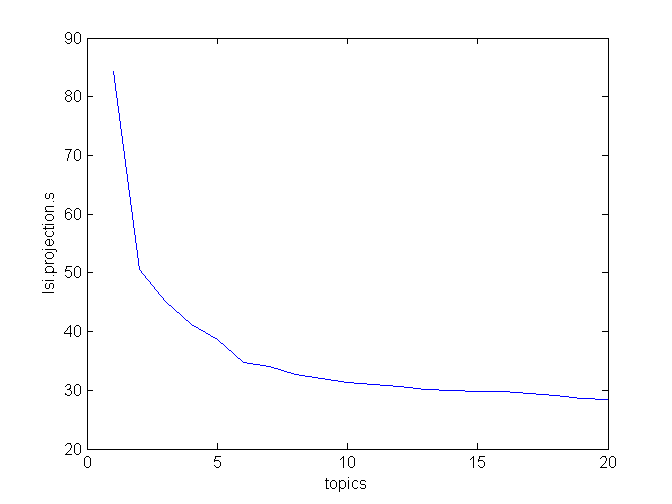
>>> lsi.projection.s
array([ 84.32124419,  50.59636515,  45.19218931,  41.2177717 ,
        38.60888714,  34.66411739,  34.10323009,  32.69769444,
        31.99280834,  31.25961344,  30.91398733,  30.60504652,
        30.16093571,  29.98871812,  29.79745159,  29.78660534,
        29.53706958,  29.11443212,  28.5729651 ,  28.36230187])

When you plot s, you notice two “elbows”, at topics = 2 and topics = 6. After that, the curve levels off.

More testing would be in order.

We would like to help Radim Rehurek, the author of Gensim, for help with the software.