Once upon a time we were browsing machine learning papers and software. We were interested in autoencoders and found a rather unusual one. It was called marginalized Stacked Denoising Autoencoder and the author claimed that it preserves the strong feature learning capacity of Stacked Denoising Autoencoders, but is orders of magnitudes faster. We like all things fast, so we were hooked.

About autoencoders

Wikipedia says that an autoencoder is an artificial neural network and its aim is to learn a compressed representation for a set of data. This means it is being used for dimensionality reduction. In other words, an autoencoder is a neural network meant to replicate the input. It would be trivial with a big enough number of units in a hidden layer: the network would just find an identity mapping. Hence dimensionality reduction: a hidden layer size is typically smaller than input layer.

mSDA is a curious specimen: it is not a neural network and it doesn’t reduce dimensionality of the input. Why use it, then? For denoising. mSDA is a stack of mDA’s, which are linear denoisers. mDA takes a matrix of observations, makes it noisy and finds optimal weights for a linear transformation to reconstruct the original values. A linear closed form solution is the secret of speed and the reason why data dimensionality must stay the same.

Apparently by stacking a few of those denoisers you can get better results. To achieve non-linear encoding, output of each layer is filtered through tanh function. This is faster than optimizing weights which have already been filtered, as in back-propagation (in case you don’t know, back propagation tends to be slow, especially in multi-layer architectures). Slowness is the Achilles’ heel of traditional stacked autoencoders.

The main trick of mSDA is marginalizing noise - it means that noise is never actually introduced to the data. Instead, by marginalizing, the algorithm is effectively using infinitely many copies of noisy data to compute the denoising transformation [Chen]. Sounds good, but does it actually work? We don’t know. We’ll see.

All in all, we don’t care that much for theory, we care for results. If it works, great. If it doesn’t, who cares for theory? So let’s find a noisy dataset and see what we can do.

The data

We’ll use Kinematics of Robot Arm dataset, described as highly non-linear and medium noisy. It comes from Luis Torgo’s regression datasets and has 8192 cases and 9 continues attributes, among them a target. Here’s a sample; we moved the target to the first column:

0.53652416,-0.015119208,0.36074091,0.46939777,1.3096745,0.98802387,-0.025492554,0.66407094,0.062762996
0.3080143,0.36047801,-0.30139478,0.62918307,-1.4401463,-0.74163685,-1.1967495,-1.0384439,-0.7174612
0.51889978,1.5632379,-1.2947529,0.078987171,1.4329368,1.1491364,-1.2921402,1.5629882,-0.93773069

It looks like data is centered around zero and nicely scaled, so we don’t have to make any decisions in this department.

We will run Spearmint to optimize two mSDA parameters: a number of stacked layers and a noise level. For now, the noise level will be the same for each layer. After denoising, we train a random forest with 400 trees, which seems to be a good value for this dataset, and give Spearmint a validation RMSE score as an error metric. We hope for smaller error after denoising.

At this point we’d better ask ourselves about how to use data for denoising. Do we denoise training and test sets together, or separately?

We suspect we’ll get better results when using both sets together. Note that we don’t use labels for denoising. This setup is certainly OK in a competition setting. In real world, it might or might not be OK.

However, what we do is basically semi-supervised learning: you learn features from unlabeled data, and only after that you build a model using those features and available labels. The point is that there is much more unlabeled data in the world than labeled data - think about images or text. In the context of robot arm data, we only have a little additional unlabeled data in the form of a test set. So we allow ourselves to use it. If it works, we might check if denoising the sets separately makes any sense.

The experiments

For starters, we will try 1-10 layers (the original paper used five) and noise in 0.01 - 0.5 range. It means that this percentage of inputs would be randomly set to zero. We mark the result with the usual colors: red the best, then green, blue and black. Here’s a Matlab snippet:

red = err < 0.139;
green = err < 0.14;
blue = err < 0.144;
black = err >= 0.144;

The code for Spearmint experiments is available at Github.

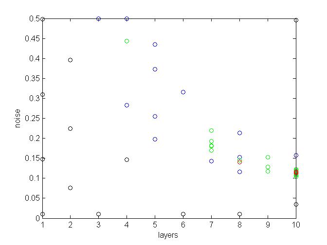
The dataset is dense, that’s why the best results are achieved with less than 15% noise. It looks like the optimal noise level is inversely correlated with a number of layers: the more layers, the less noise needed. It is also plain to see that when testing up to 10 layers, the more layers, the better. Therefore in the next run we will test settings with even more layers.

But first, let’s check one thing. Would varying a noise in each layer help? We will use ten layers and optimize noise separately for each layer - so that there is 10 hyperparams to tune now. This is a mean of good run settings (noise levels from all good runs, averaged by layer):

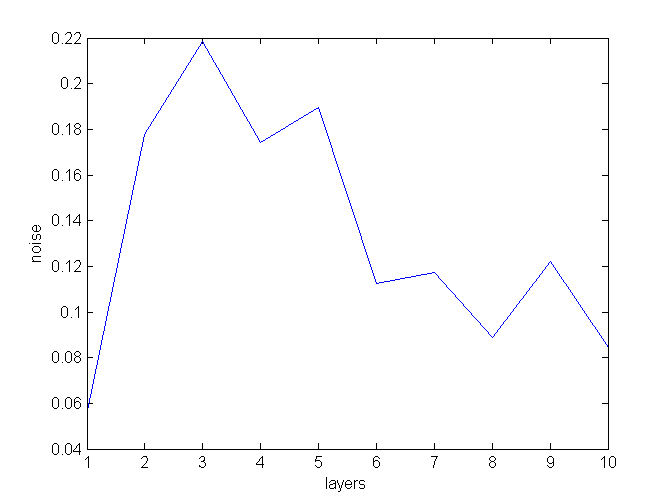
It looks like Spearmint thinks that this shape is most promising. To summarize:

• first layer: low noise
• layers 1-5: high noise
• layers 6-10: medium noise

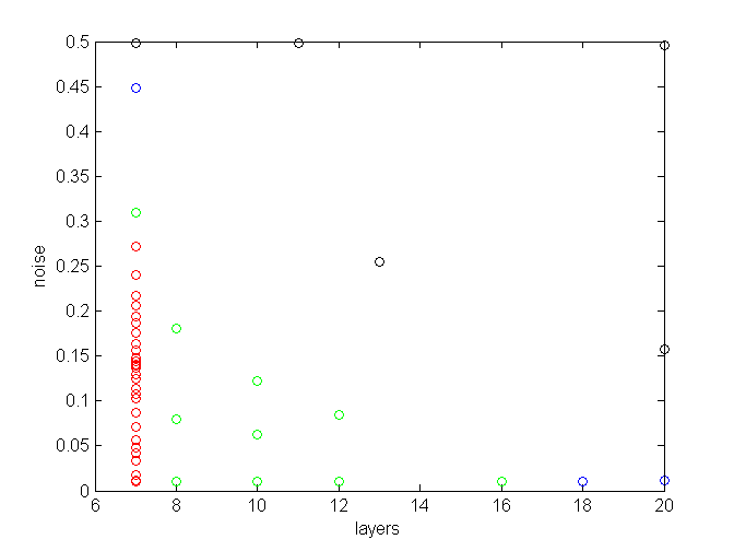
However, in 69 tries we didn’t exceed the best results from the constant scenario. It may be that we need more tries to optimize ten hyperparams, but for now it seems that varying noise isn’t going to give us any mega-improvements, so we’ll stick with the simpler constant noise model. Let’s see how it goes with more layers:

From the second run we conclude that there are several good settings for layers and noise, provided that there is at least 10 layers. We chose 14 layers and a noise of 0.06 as the optimal setting used for testing. What’s important is to consider the two hyperparams together, because optimal noise for 10 layers will differ from optimal noise for 14 layers.

So does it work? On a test set we get RMSE = 0.142 for a random forest trained on original data, and 0.136 after training on denoised data. This means that there is an improvement after denoising. It would be nice to investigate further.

A possible variation is to use original and denoised features together. It doesn’t work in this case, as it produced an error = 0.232.

UPDATE

However, as Andy points out in the comments, better results can be achieved by feeding all layers to a random forest. That is, not only original and final denoised features, but intermediate layers as well. Andy reports getting 0.1288 in the first try and 0.128 after letting Spearmint run for a while. With variable noise it’s better still: 0.127 after 10 Spearmint iterations.

The modification is simple: just comment one line in run_denoise.m:

x2 = allhx';
% x2 = x2(:, start_i:end_i );       % <--- this one

Of course, the dimensionality goes up: ten times with ten layers. In case of low-dimensional datasets like kin8nm it is not a problem. Otherwise you might consider trying out a linear model.

What about linear regression instead of random forest?

Most of the time in optimizing is spent learning random forest models. The question that may come to mind is whether training a simpler model, like regularized linear regression, would lead to selecting the same, or at least similiar, hyperparam values? If so, we could optimize much faster.

Unfortunately the answer is no. We trained a ridge regression model instead of random forest, and it seems that it prefers different params altogether, specifically less layers:

By the way, best RMSE achieved was about 0.2, which we consider pretty good for a linear model. The conclusion is that if we want to use a random forest for predicting, we need to optimize mSDA hyperparams for a random forest.