We present a novel method for feature transformation, akin to standardization. The method comes from Michael Jahrer, who recently has won another competition and afterwards shared the approach he used.

There are a few things of general interest in the write-up. For example, it confirms once again that gradient boosting is much faster and much easier to use than neural networks while delivering similar results. Michael used lightgbm:

Nice library, very fast, sometimes better than xgboost in terms of accuracy. One model in the ensemble. I tuned params on CV.

For neural networks, Jahrer proposes a non-standard method that apparently worked better than standardization or normalization. He calls it RankGauss:

Input normalization for gradient-based models such as neural nets is critical. For lightgbm/xgb it does not matter. The best what I found during the past and works straight of the box is “RankGauss”. Its based on rank transformation.

First step is to assign a linspace to the sorted features from -1…1, then apply the inverse of error function ErfInv to shape them like gaussians, then I substract the mean. Binary features are not touched with this trafo (eg. 1-hot ones). This works usually much better than standard mean/std scaler or min/max.

Even though the name RankGauss reflects the order of the two steps of the method, we prefer “GaussRank”. It sounds better.

To implement it, first we compute ranks for each value in a given column (argsort). Then we normalize the ranks to range from -1 to 1. Then we apply the mysterious erfinv function. The purpose of this is to make the distribution of the transformed ranks Gaussian.

Actually, erfinv(-1) is -inf and erfinv(1) is inf, so we need to account for that.

import numpy as np
import matplotlib.pyplot as plt

from scipy.special import erfinv

# simulating normalized ranks from -0.99 to 0.99
x = np.arange( -0.99, 1, 0.01 )

y = erfinv( x )
plt.hist( y )

Subtracting the mean isn’t really necessary as it is very close to zero.

In [33]: y.mean()
Out[33]: 1.7495775905650709e-15

In practice

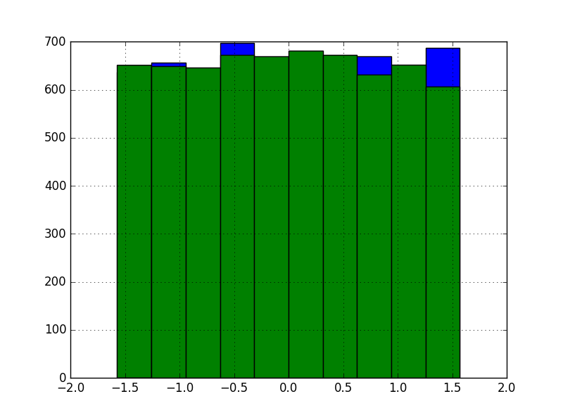
To learn how it works, we tested the method on the kin8nm dataset. Features in the dataset, eight total, are distributed more or less uniformly. Here’s a histogram of the first two in the training set:

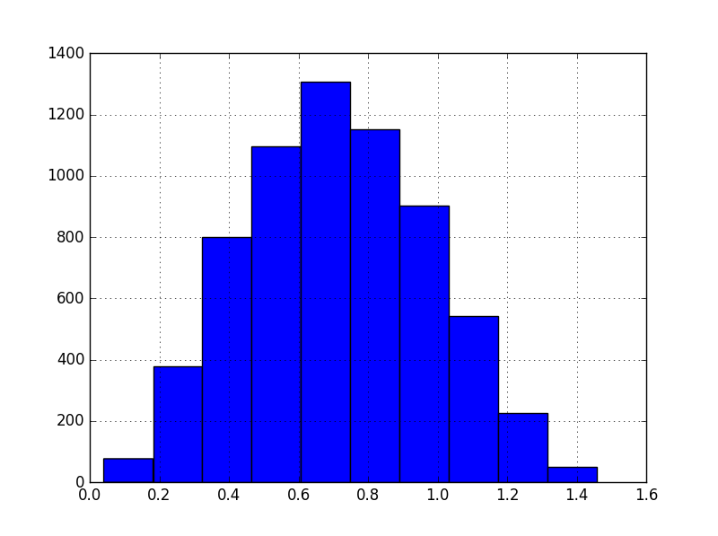
In contrast, the target variable:

We implemented fit_predict() method for GaussRank, since it’s much easier than writing separate fit() and predict() methods. The way to use it to take the features both from the training and the testing sets and fit/transform then jointly. It is OK, because we’re not using any labels.

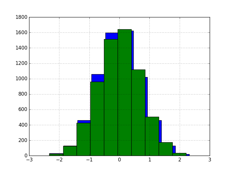
The histogram of the first two features after transformation:

For neural networks we used Keras and performed a hyperparam search with Hyperband, for two versions of the dataset: with and without GaussRank.

The best score we obtained with the original version was 8.14% RMSE, which is close to what we achieved with PyBrain a while ago. For the transformed version, it was 10.86%. Therefore we must conclude that GaussRank does not work well with the dataset.

For comparison, we also transformed the data with random projections, keeping the same dimensionality. Note that this method transforms the X matrix as a whole, instead of column-by-column scheme of GaussRank.

This version yielded even more unimpressive 13.27% RMSE. This is no surprise, because unsupervised random projections are in general unlikely to result with better representation for supervised learning.

Data, code and results for the experiments are available on GitHub.