Object recognition in images is where deep learning, and specifically convolutional neural networks, are often applied and benchmarked these days. To get a piece of the action, we’ll be using Alex Krizhevsky’s cuda-convnet, a shining diamond of machine learning software, in a Kaggle competition.
Continuing to run things on a GPU, we turn to applying convolutional neural networks for object recognition. This kind of network was developed by Yann LeCun and it’s powerful, but a bit complicated:
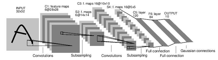
Image credit: EBLearn tutorial
A typical convolutional network has two parts. The first is responsible for feature extraction and consists of one or more pairs of convolution and subsampling/max-pooling layers, as you can see above. The second part is just a classic fully-connected multilayer perceptron taking extracted features as input. For a detailed explanation of all this see unit 9 in Hugo LaRochelle’s neural networks course.
Daniel Nouri has an interesting story about applying convnets to audio classification. His insight:
Convnets can have hundreds of thousands of neurons (activation units) and millions of connections between them, many more than could be learned effectively previously. This is possible because convnets share weights between connections, and thus vastly reduce the number of parameters that need to be learned.
As regards software, we could use pylearn2, but let’s try something else for a change: cuda-convnet, a fast implementation of feed-forward neural networks in C++/CUDA/Python. Its author, Alex Krizhevsky, is also the main creator of a popular benchmark dataset for object recognition: CIFAR-10. The set is a collection of 32x32 color images of cats, dogs, cars, trucks etc. - a total of 10 object classes.
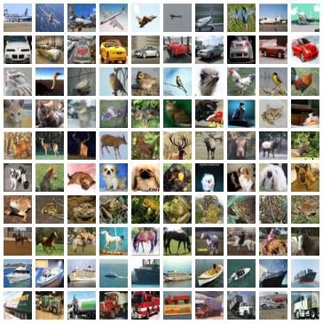
It happens that there’s a Kaggle competition based on CIFAR-10. The training set is the same, the test set images are modified and buried among 290k other images to discourage cheating.
Running cuda-convnet
Our impression is that cuda-convnet feels more solid and tidy than pylearn2, and also quicker. It’s certainly more specialized.
Here’s a snippet of training output:
1.1... logprob:  2.151354, 0.798000 (64.006 sec)
1.2... logprob:  1.886476, 0.693500 (13.407 sec)
1.3... logprob:  1.723293, 0.634800 (13.403 sec)
1.4... logprob:  1.678299, 0.613200 (13.400 sec)
2.1... logprob:  1.600135, 0.581400 (13.403 sec)
The first number is epoch, the second - batch. The software saves the model every x batches, so it’s possible to hit Ctrl-C and resume later. Then goes log probability, training error and time taken for the batch. We used a notebook with GeForce GT 650 M, as in CUDA on a linux laptop.
You can inspect training results using shownet.py.
Worth mentioning is noccn, a collection of wrappers around cuda-convnet by Daniel Nouri. The author also provides a version of cuda-convnet with dropout. Noccn can be used to make batches and produce predictions, although it’s a tiny bit complicated so for the purposes of the task at hand we chose to roll out some simpler code.
Our scripts are available at Github. Aside from cuda-convnet, you’ll need natsort module in Python. We use it to sort image names so that 2.png is before 10.png.
Images into batches
As usual, we need to figure out how to get data in and predictions out. Kaggle provides PNG images, while cuda-convnet expects data in form of batch files. A batch file is a pickled Python dictionary containing at least image data and labels. CIFAR batches are 10000 images each.
from PIL import Image
image = Image.open( '1.png' )
Now the question is, how to convert it into a Numpy array? Turns out to be easy:
image = np.array( image )           # 32 x 32 x 3
image = np.rollaxis( image, 2 )     # 3 x 32 x 32
image = image.reshape( -1 )         # 3072
What follows the first line is to make data compatible with cuda-convnet format. Data for each RGB channel goes separately, so we need to move that axis to the front before reshaping.
You can verify that it works by loading a train batch and printing the first row from the data array. Then you load the corresponding PNG image, process it as above, print the resulting array and compare to the original.
Let’s make test batches:
python make_test_batches.py <images dir> <output dir>
python make_test_batches.py test test_batches
We end up with 30 new batches that we’d like predictions for.
The predictions
How do you get predictions from cuda-convnet? It’s under-documented, but fortunately there’s a way. The software has a feature for writing features from a chosen layer. When you write features from the softmax layer (named probs in the layer definition file), you get probabilities for each class. They are saved in a batch file somewhat similiar to the training batches. The relevant command line options are:
shownet.py -f <path to model dir> --write-features=probs --feature-path=/path/to/predictions/dir --test-range=7-36
But wait… We followed the procedure for training the model with 13% test error. It uses 24x24 patches for training and for testing:
After training is done, you can kill the net and re-run it with the –test-only=1 and –multiview-test=1 arguments to compute the test error as averaged over 10 patches of the original images (4 corner patches, center patch, and their horizontal reflections). This will produce better results than testing on the center patch alone.
With multiview you get 12.6% error, without it - 15.4%. It seems that we’re going to use multiview predictions from noccn. We copied the appropriate functions to the modified shownet.py script.
shownet.py -f <path to model dir> --write-predictions=/path/to/predictions/file --test-range=7-36 --multiview-test=1
Afterwards we unpickle the file and for each example get an index of the most probable class:
label_names = [ 'airplane', 'automobile', 'bird',  'cat', 'deer', 'dog', 'frog', 'horse', 'ship', 'truck' ]
# mapping from indexes to names
labels_dict = { i: x for i, x in enumerate( label_names ) }

d = pickle.load( open( batch_path, 'rb' ))
label_indexes = np.argmax( d['data'], axis = 1 )    # data is 300000 x 10

for i in label_indexes:
    label = labels_dict[i]
This code is in the predict_multiview.py script, here’s how to run it:
python predict_multiview.py pickled_predictions_file predictions.csv
And indeed, we get 0.8756 on the leaderboard.
Online image classification demos
If you’d like your own image classified, try these online demos:
By the way, we post such tidbits on Twitter, so consider following @fastml_extra.