Out of 215 contestants, we placed 8th in the Cats and Dogs competition at Kaggle. The top ten finish gave us the master badge. The competition was about discerning the animals in images and here’s how we did it.
We extracted the features using pre-trained deep convolutional networks, specifically decaf and OverFeat. Then we trained some classifiers on these features. The whole thing was inspired by Kyle Kastner’s decaf + pylearn2 combo and we expanded this idea. The classifiers were linear models from scikit-learn and a neural network from Pylearn2. At the end we created a voting ensemble of the individual models.
OverFeat features

We touched on OverFeat in Classifying images with a pre-trained deep network. A better way to use it in this competition’s context is to extract the features from the layer before the classifier, as Pierre Sermanet suggested in the comments.
Concretely, in the larger OverFeat model (-l) layer 24 is the softmax, at least in the version we’d been using, which seems to be 3.2. You can see that by extracting features from this layer: they are 1000-dimensional, and that’s the number of ImageNet classes:
$ cd data
$ path/to/overfeat -l -L 24 train/cat.1.jpg | head -1
1000 1 1
By the way, the meaning of “layer” here is not the usual one, because an OverFeat layer refers to things like non-linear activation too. For example, layer 23 is a rectifier activation. You can see this by comparing features from layer 22 and 23. The latter differ from the former only by replacing negative values with zero:
$ overfeat -l -L 22 train/cat.1.jpg
4096 1 1
-0.800539 -1.8362 -0.567662 -5.75431 -3.17502 -1.92718 -2.15222 -1.94303 0.6074 -4.51182 (...)

$ overfeat -l -L 23 train/cat.1.jpg
4096 1 1
0 0 0 0 0 0 0 0 0.6074 0 (...)
The same goes to layers 20 and 21. We extracted the features from layer 22 and 20. Both were good. The layers below 20 produce bigger windows and we didn’t try them.
OverFeat is able to handle images of different shapes and size. The number of features, or more accurately, feature maps is set in the model, but the dimensionality of the maps (windows) depends on image shape. The top layers will yield 1x1 windows for square images, 1xn windows for “horizontal” images and nx1 windows for “vertical” images:
$ cd overfeat
$ ./bin/linux/overfeat -l -L 22 samples/bee.jpg | head -1
4096 1 4
$ ./bin/linux/overfeat -l -L 22 samples/stairs.jpg | head -1
4096 4 1
This begs the question of how to use the features from non-square images. One solution would be to crop the images square to get 1x1 features. Another, better one, is to take the max value from each window as a feature. This is what convolutional networks do in pooling layers and it’s called max-pooling. One way to implement it in Numpy:
# after reading dims from the file's first line...
data = np.loadtxt( f, skiprows = 1 )

data = np.reshape( data, dims )             # 1D to 3D
data = np.amax( np.amax( data, 1 ), 1 )     # max over columns and rows
After max-pooling you get 4096 scalar features for each image.
Classifying
The high number of dimensions suggests a linear classifier. We used a logistic regression model from scikit-learn. It has one hyperparam, C, the [inverse] strength of regularization. Following Daniel Nouri’s suggestion, we used a value of 0.001. It seemed to offer the best performance in validation.
Scikit-learn has another linear model for classification: a passive-agressive perceptron. It has one additional hyperparam, a number of iterations. More iterations lead to overfitting, so you need to balance it with regularization.
Come to think of it, there are also various flavours of linear discriminant analysis and linear SVM, didn’t try them.
Standardizing
A question you may ask yourself: what about standardization, that is scaling the features and subtracting the mean? We tried that and generally the validation scores were slightly worse than from raw features.
from sklearn.preprocessing import StandardScaler

scaler = StandardScaler()
x = scaler.fit_transform( x )
Only in case of logistic regression with decaf features scaling helped a tiniest little bit (< 0.1% accuracy), even though the columns had definitely non-zero means and non-unit standard deviations. The output shows min/avg/max over the columns:
standardizing x...
min/avg/max scaler.mean_: -61.310459137 / -17.8648929596 / 2.22160768509
min/avg/max scaler.std_: 11.0898637772 / 15.7399768829 / 25.3764019012
As regards OverFeat layer 22 features, they were better behaved already:
min/avg/max scaler.mean_: -3.51754036999 / -1.30101070252 / 1.24087636685
min/avg/max scaler.std_: 0.856160182276 / 1.66191373533 / 3.37190837123
Layer 20 was slightly wilder, but still did better without standardizing:
min/avg/max scaler.mean_: -8.63044079365 / -2.86932641897 / 1.59710002958
min/avg/max scaler.std_: 0.948877928982 / 2.96835429318 / 5.29119926156
Bagging
At this point we have three sets of features: one from decaf and two from OverFeat layers 20 and 22. You can combine two or three sets into one with even higher dimensionality. We also have a few models for each set: Pylearn2 NN, LR and PAC. This leads to a number of predictions. We bagged them in the form of a voting ensemble.
Each model predicts either one or zero. We took predictions from nine models. If the row sum was bigger than four, we considered the prediction positive, otherwise negative. This procedure is simple and assumes that each model is equally good. That’s not quite true, but spread of validation scores was roughly 0.97 to 0.98, so they’re reasonably close. A better, but more complicated way, would be to weigh the models by their scores using predictions from a separate validation set.
Bagging seemed to up the score on the public part of the test set to ~0.875 from ~0.87 for the best single model. We didn’t submit many, the best happened to be OverFeat 22 + Pylearn2.
Here are sample images about which the ensemble members disagreed the most, some rescaled:


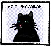


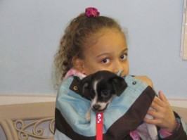

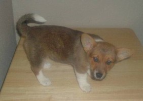
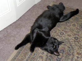
Some are harder - “no photo available” appeared four times - some seem to be straightforward. Now, what about this guy?
Image credit: @HistoricalPics