AUC, or Area Under Curve, is a metric for binary classification. It’s probably the second most popular one, after accuracy. Unfortunately, it’s nowhere near as intuitive. That is, until you have read this article.

Accuracy deals with ones and zeros, meaning you either got the class label right or you didn’t. But many classifiers are able to quantify their uncertainty about the answer by outputting a probability value. To compute accuracy from probabilities you need a threshold to decide when zero turns into one. The most natural threshold is of course 0.5.

Let’s suppose you have a quirky classifier. It is able to get all the answers right, but it outputs 0.7 for negative examples and 0.9 for positive examples. Clearly, a threshold of 0.5 won’t get you far here. But 0.8 would be just perfect.

That’s the whole point of using AUC - it considers all possible thresholds. Various thresholds result in different true positive/false positive rates. As you decrease the threshold, you get more true positives, but also more false positives. The relation between them can be plotted:

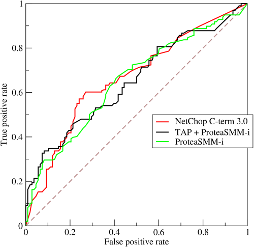
Image credit: Wikipedia

From a random classifier you can expect as many true positives as false positives. That’s the dashed line on the plot. AUC score for the case is 0.5. A score for a perfect classifier would be 1. Most often you get something in between.

Computing AUC

One computes AUC from a vector of predictions and a vector of true labels. Your favourite environment is bound to have a function for that. A few examples:

• In Python, there’s scikit-learn with sklearn.metrics.auc, or rather sklearn.metrics.roc_auc_score
• In Matlab (but not Octave), you have perfcurve which can even return the best threshold, or optimal operating point
• In R, one of the packages that provide ROC AUC is caTools
• Ben Hamner’s Metrics has C#, Haskell, Matlab, Python and R versions

Finer points

Let’s get more precise with naming. AUC refers to area under ROC curve. ROC stands for Receiver Operating Characteristic, a term from signal theory. Sometimes you may encounter references to ROC or ROC curve - think AUC then.

But wait - Gael Varoquaux points out that

AUC is not always area under the curve of a ROC curve. In the situation where you have imbalanced classes, it is often more useful to report AUC for a precision-recall curve.

ROC AUC is insensitive to imbalanced classes, however. Try this in Matlab:

y = real( rand(1000,1) > 0.9 );  % mostly negatives
p = zeros(1000,1);               % always predicting zero
[X,Y,T,AUC] = perfcurve(y,p,1)   % 0.5000

That’s another advantage of AUC over accuracy. In case your class labels are mostly negative or mostly positive, a classifier that always outputs 0 or 1, respectively, will achieve high accuracy. In terms of AUC it will score 0.5.

The same goes to random predictions:

y = real( rand(1000,1) > 0.1 );  % mostly positives
p = rand(1000,1);                % random predictions
[X,Y,T,AUC] = perfcurve(y,p,1)   % 0.4996
plot(X,Y)

y = real( rand(1000,1) > 0.9 );  % mostly negatives
p = rand(1000,1);                % random predictions
[X,Y,T,AUC] = perfcurve(y,p,1)   % 0.4883
plot(X,Y)   

And zero zero seven, there’s one more thing you need to know about AUC: it doesn’t care about absolute values, it only cares about ranking. This means that your quirky classifier might as well output 700 for negatives and 900 for positives and it would be perfectly OK for AUC, even when you’re supposed to provide probabilities. If you need probabilities, use a sigmoid, but remember: for AUC it doesn’t make any difference.