Very often performance of your model depends on its parameter settings. It makes sense to search for optimal values automatically, especially if there’s more than one or two hyperparams, as is in the case of extreme learning machines. Tuning ELM will serve as an example of using hyperopt, a convenient Python package by James Bergstra.
Updated November 2015: new section on limitations of hyperopt, extended info on conditionals.
Software for optimizing hyperparams
Let’s take a look at software for optimizing hyperparams. These are the notable packages that we know of (we covered Spearmint a while ago):
- Spearmint (Python)
- BayesOpt (C++ with Python and Matlab/Octave interfaces)
- hyperopt (Python)
- SMAC (Java)
- REMBO (Matlab)
- MOE (C++/Python)
The authors of SMAC also have HPOLib, a common interface to SMAC, Spearmint and Hyperopt, and Auto-WEKA. Then there is adaptive resampling in caret and randomized parameter optimization in scikit-learn. Finally, you’ll find a few more links in MOE docs.
We have tried the first three from the list above. Spearmint and BayesOpt use Gaussian processes. One issue with GPs is that you have to choose priors. This is especially pronounced in case of BayesOpt: it looks like you need to tune hyperparams for the hyperparam tuner.
Spearmint takes care of this problem, but is slow: it takes a few minutes to tune the benchmark Branin function, while hyperopt takes just a few seconds. On the other hand, Spearmint’s overhead matters less with objective functions which run longer, e.g. for an hour. And Spearmint finds the optimal solution for Branin in roughly 35 function evaluations, while hyperopt needs twice as much.
Hyperopt also uses a form of Bayesian optimization, specifically TPE, that is a tree of Parzen estimators. If you’re interested, details of the algorithm are in the Making a Science of Model Search paper.
Hyperopt limitations
It’s not possible to continue beyond the initially chosen number of experiments or to use any information from previous experiments, as MOE does. In addition, you can’t pause, save, and later load and resume, although this is a property of the implementation, not the underlying algorithm.
However, Brent Komer says that hyperopt also does have the ability to save and later load and resume. This is done via the “Trials” object. We’re not convinced for now.
As the authors note in the paper on optimizing convnets,
The TPE algorithm is conspicuously deficient in optimizing each hyperparameter independently of the others. It is almost certainly the case that the optimal values of some hyperparameters depend on settings of others. Algorithms such as SMAC (Hutter et al., 2011) that can represent such interactions might be significantly more effective optimizers than TPE.
This means that if you have parameters that obviously depend on each other, you might try fixing one at a reasonable value and letting the library experiment with the other(s). One such scenario is learning rate settings, which usually consist of at least initial learning rate and one or more decay parameters.
The process
The main things to do are:
- describe the search space, that is hyperparams and possible values for them
- implement the function to minimize
- optionally, take care of logging values and scores for analysis
The function to minimize takes hyperparam values as input and returns a score, that is a value for error (since we’re minimizing). This means that each time the optimizer decides on which parameter values it likes to check, we train the model and predict targets for validation set (or do cross-validation). Then we compute the prediction error and give it back to the optimizer. Then again it decides which values to check and the cycle starts over.
Spearmint will search indefinitely, so it’s your call to stop. With hyperopt, on the other hand, you decide how many iterations you’d like to run. One needs to give the optimizer enough tries to find near-optimal results. 50-100 iterations seems like a good initial guess, depending on the number of hyperparams.
Conditionals
Perhaps the most interesting feature of hyperopt is support for describing alternative scenarios. Let’s say, for example, that you’d like to tune a neural network. How many hidden layers to use? With software like Spearmint, which doesn’t allow conditionals, you’d be forced to run a separate experiment for each option. That’s because parameters for the second layer will be meaningless if there’s only one layer in the particular test; it could confuse the optimizer. The solution:
space = {
    'layer_1_size': hp.qloguniform( 'layer_1_size', log( 2 ), log( 1e4 ), 1 ),

    'layer_2': hp.choice( 'layer_2', [
        False,
        {
            'layer_2_size': hp.qloguniform( 'layer_2_size', log( 2 ), log( 1e4 ), 1 )
        }
    ]),
    ...
}
With hyperopt’s choice you can specify sophisticated structures, for example test two classifiers, each with its own set of hyperparams. This example is adapted from the hyperopt’s docs:
space = hp.choice('classifier_type', [
    {
        'type': 'naive_bayes',
    },
    {
        'type': 'svm',
        'C': hp.lognormal('svm_C', 0, 1),
        'kernel': hp.choice('svm_kernel', [
            {'ktype': 'linear'},
            {'ktype': 'RBF', 'width': hp.lognormal('svm_rbf_width', 0, 1)},
        ]),
    }
])
Naive Bayes has no hyperparams to tune, while SVM have a few, including the choice of a kernel.
Parameter ranges
When you have a numeric parameter to optimize, the first question is: discrete or continuous? For example, a number of units in a neural network layer is an integer, while amount of L2 regularization is a real number.
A more subtle and maybe more important issue is how to probe values, or in other words, what’s their distribution. Hyperopt offers four options here: uniform, normal, log-uniform and log-normal.
Let’s use an example to understand the importance of log distributions: for some params, like regularization, the distinction among small values is important. Maybe we think the range for regularization param should be 0 to 1, but most likely it will be a small value like 0.01 or 0.001. Therefore we don’t want the optimizer to probe the range uniformly, because it would waste time trying to distinguish between 0.4 and 0.6 when in fact there’s not much difference, because both these values are too big.
Instead we use the log-uniform, or possibly log-normal distribution so that the optimizer could make fine distinctions with small values. We describe the log-uniform distibution below in more detail.
Log-uniform distribution
Here’s some Matlab/Octave code to visualize a log-uniform distribution:
u = rand( 100000, 1 );
bins = 20;
hist( u, bins )
hist( exp( u ), bins )
hist( exp( u * 5 ), bins )


You can see that exponential/log-uniform distribution can have a heavier or a lighter tail, but either way smaller values are more common.
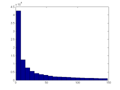
The search space
This table of hyperparams to optimize might give you an idea what log-uniform distribution is good for:
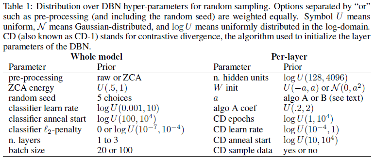 Source: Algorithms for Hyper-Parameter Optimization [PDF].
And here’s our search space definition for ELM:
space = (
    hp.qloguniform( 'n_hidden', log( 10 ), log( 1000 ), 1 ),
    hp.uniform( 'alpha', 0, 1 ),
    hp.loguniform( 'rbf_width', log( 1e-5 ), log( 100 )),
    hp.choice( 'activation_func', [ 'tanh', 'sine', 'tribas', 'inv_tribas', \
        'sigmoid', 'hardlim', 'softlim', 'gaussian', \
        'multiquadric','inv_multiquadric' ] )
)
With log-distributions we need to supply log()s of parameter value limits - doing so explicitly allows us to think in natural ranges of values. The number of hidden units is a discrete quantity so we use the qloguniform option.
Logging the results
After optimization is complete we’d like to look at settings explored and scores achieved, so we save them to a file. We have a wrapper function which takes care of that. We pass the wrapper function to hyperopt, the wrapper calls the proper function, saves the params and the result and returns the error value to hyperopt.
Hyperopt also has the Trials class that serves the same purpose. if you pass an object of this class, say trials, to fmin(), at the end it will contain information about params used, results obtained, and possibly your custom data.
The data
We will use ELM on the data from Burn CPU burn competition at Kaggle. The goal is to predict CPU load on a cluster of computers. There are less than 100 columns, mostly numeric, with the exception of timestamps and machine IDs (there’s seven computers). We treat the machine ID as a categorical variable. A more complicated alternative would be to build a separate model for each computer, however some quick tests of this approach showed worse results.
There are roughy 180k examples, sorted by time. We take the first 93170 as the training set and set aside the remaining 85610 points for validation. This is meant to mimic the original train/test split.
Lessons learned
ELM involve randomness, meaning that with the same hyperparams the error will differ - hopefully slightly - from run to run. We need to account for this in optimizing the parameters and the way to do this is to run each setting a few times and average the results. We missed this point initially so the scripts run each setting just once. Luckily it doesn’t seem to make that much difference in this case.
Here are a few more points (regarding this specific dataset, possibly generalizing to other):
Standardize data first. We were reluctant to standardize one-hot indicator columns for categorical variables, but it seems it’s better to standardize them too.
Pipeline setup runs faster than normal ELM, probably because Ridge is faster than ELM’s built-in linear model.
Ridge also offers a better performance in terms of score.
Rectified linear activation seems to work just as well as other functions (RMSE 4.8 in validation)
The results from two hidden layers are basically the same as with one hidden layer.
There are different hyperparam combinations resulting in similiar performance. You can bag the models. We bagged a few models and got a slight improvement, from RMSE roughly 4.8 to 4.4 in validation.
Predictions from the best pipeline/Ridge model score 5.13 on the public leaderboard.
Complete code is available at GitHub.